
Dispersion Trading Part 2
- Noel Smith, Leo Capalleja & Sebastian Pachon

- Jul 10, 2023
- 6 min read
Updated: Aug 19, 2024
In this second part of a series we will explain what implied volatility is and why it matters for option valuation. We will then connect this concept to dispersion trading and show the importance of expected vs. realized outcomes. Finally, we will discuss some additional features of dispersion trading.
Volatility Expectations vs Reality
Trading is a matter of expectations versus actual events. When traders buy or sell assets, they make decisions based on what they think is going to happen in the future. We discussed in the first article of this series a long dispersion trade is a way to benefit from low correlation between the components of an index. This means that if we hold a position like this, our expectation is that the moves of the stocks within an index will be less correlated than the market implies.
There is an important concept that should be discussed before explaining more details about dispersion trading, and that is implied volatility. To price an equity option, we need the following parameters:
From the list above, σ is the only input that is not known at time zero, and different values of σ will impute different option prices. As an example, consider a stock XYZ that currently trades at $100 and has a dividend yield of 1%. Assume the risk-free rate, r, is 3%. Using Black-Scholes-Merton formulas, a 1-year European call option with strike $100 and a 30% volatility will cost $12.69. On the other hand, if instead of using 30% volatility we use 40%, the call price rises to $16.54, a 30% increase. Note that for both of these cases there is an assumption of the future realized volatility for stock XYZ. This means that for different views (or expectations) of volatility, there will be different option prices.
In the real world, this “subjectiveness” in option pricing is avoided by not guessing any volatility at all, and simply extracting it from where the market is trading. Hence, will not be treated as a known input, but as a market-implied one. Continuing with our previous XYZ call option example, assume now that we see that the price to buy it is $10.88 (everything else held constant). We can be confident that its expected volatility is now lower than 30%, given that for =30% the call is worth $12.69, and $10.88 is lower than $12.69. So, the question is: What volatility should we input into the pricing formula to get a price of $10.88? Put differently, what is the implied volatility for this option? The answer is 25.3%, which represents the implied volatility that the market is expecting for XYZ over the following year. Note that the methods used to solve for the implied volatility are beyond the scope of this paper but many calculators are available online.
Implied volatility is crucial for options trading, and hence, for dispersion trading. If we expect that the future volatility of XYZ will be above (below) 25.3% we can buy (sell) the option for $10.88. The P/L of this trade will largely depend on the realized volatility of XYZ after we enter our position. Generally, the trade will profit if the realized volatility is above (below) 25.3% and lose if the realized volatility is below (above) 25.3%.

Implied Volatility in the Dispersion Trade
Now, let’s connect the previous concepts to dispersion. From now on, we will be using the same three example assets that were introduced in our previous article: stock A, stock B and index AB. If we want a long dispersion position, we will have to buy 0.5 units of notional in a straddle for stock A, buy 0.5 units of notional in a straddle for stock B and sell 1 unit of notional in a straddle for index AB. Just like the XYZ call example before, we can describe the P/L of this trade by comparing the implied volatility of the options at the time of the trade to the future realized volatility of stock A, stock B and index AB.
The following scenarios will be helpful to describe the performance of a dispersion strategy under different environments. In this scenario comparison, we first make an assumption of future returns for A, B and AB (unknown at the time the trade is initiated). We then compute proxies for P/L based on different starting implied volatilities (i.e. different prices).
Assume that the 1-year returns of the three assets were:
Stock A: +10%
Stock B: -4%
Index AB: +3%
Scenario 1 – Higher realized volatility than expected.
At time zero, when we placed the trade and bought/sold the straddles, we had:
Stock A implied volatility of 7%
Stock B implied volatility of 2%
Index AB implied volatility of 5%
The following computation would give us a proxy of the P/L:
0.5 x (|10%| - 7%) + 0.5 x (|-4%| - 2%) - 1.0 x (|3%| - 5%) = 1.5% + 1.0% + 2.0% = +4.5%
This is an excellent scenario. The realized movement was higher than expected for our long positions (stocks A and B) and lower than expected for our short position (index AB). In this scenario we profit from both our long and short positions.
Scenario 2 – Lower realized volatility than expected.
At time zero, when we placed the trade and bought/sold the straddles, we had:
Stock A implied volatility of 12%
Stock B implied volatility of 6%
Index AB implied volatility of 3%
Using the same formula as before:
0.5 x (|10%| - 12%) + 0.5 x (|-4%| - 6%) - 1.0 x (|3%| - 3%) = -1.0% - 1.0% + 0.0% = -2.0%
Opposite from the previous example, this is a losing scenario. The realized movement was lower than expected for our long positions and equal to expectations for our short position. In this scenario we lose on our long position and break even on our short position.
Introduction to Implied Correlation
Having shown these examples and definitions, we now introduce a generalization of dispersion. Consider an index that is composed of n components. We define the spot price and implied variance of a basket of n stocks as:
Where:
Note that the pairwise implied correlation terms in the variance formula, ρ, are not possible to compute directly. However, we can rearrange the terms of the variance equation above to solve for the pairwise implied correlation term and relabel it as the weighted-average pairwise implied correlation (or “implied correlation” for short).
Just as implied volatility provides options traders insight into the expected future volatility of a stock, implied correlation gives dispersion traders insight into the expected future correlation of the components of an index.
Why does dispersion trading work and what drives an opportunity like this?
Financial institutions, such as asset managers, pension funds and insurance companies, are permanently buying protection against downturns in the market through put options. From a simple supply/demand perspective, this constant bid for put options will drive implied volatilities higher at the index level. This causes index implied volatilities to trade at a premium in comparison to their future realized movements.
In contrast, single-name stock options are popular amongst investors as yield enhancement vehicles. Investors will often sell covered calls on their positions or write cash-secured puts on stocks they would like to add to their portfolios. This applies a slight downward pressure on single-name stock’s implied volatilities.
The combination of the aforementioned dynamics generates an opportunity to sell index volatility (usually trading at a premium) and buy individual stock volatility (usually trading at a discount or at fair-value). This is precisely what dispersion trading is benefiting from and the reason for an opportunity like this to exist.
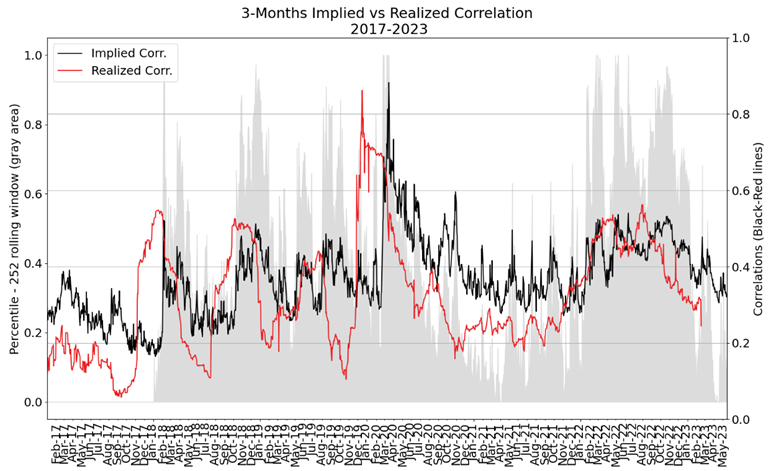
Historical data shows how implied correlation typically trades at a premium to realized correlation. In other words, and similar to what happens between implied volatility and realized volatility, the market's expectations of individual stock correlations tend to under-realize.
Lastly, one large but unpredictable benefit of dispersion trading is luck. This is due to dispersion portfolios being long single-name stock options and unexpected idiosyncratic events taking place for those stocks. Examples of such events are: scandals, take-overs, buyouts, lawsuits, balance sheet blowouts (think SVB in 2023), natural disasters, etc. Any large single-name move up or down that manifests from unexpected news can add significant profitability to a dispersion portfolio. And since dispersion books in this form are inherently long options this is a serendipitous event can not be predicted but definitely adds to profit.
Convex Asset Management LLC emphasizes that investing in futures, options, and other derivatives involves substantial risk and is not suitable for all investors. There is a possibility that you may sustain a significant loss, including a complete loss of your investment capital. Past performance is not necessarily indicative of future results. Investing involves risks, and any investment strategy carries the risk of loss. Before investing, carefully consider your financial objectives, level of experience, and risk tolerance. You should only invest funds that you can afford to lose and seek independent financial advice if you have any concerns or questions.

Implied Correlation formula has the term "basket variance" which uses implied correlation between two stocks (rho). How to calculate that? Thanks.